

What do you need to estimate laser cutting time?
For a first estimate, divide cutting length by the applicable feed rate, then add piercing, non-cutting moves and other program actions. A useful estimate identifies the source of each input and the moment its clock starts and stops.
Here, program time runs from cycle start to program end on a sheet already loaded and ready to cut. Keep material retrieval, loading, sorting and inspection in separate records so you can add them when planning the whole order.
| Input | What to record |
|---|---|
| Drawing and quantity | DXF revision, required parts and the nest being estimated. |
| Material and cutting conditions | Grade, thickness, surface condition, laser power and assist gas. |
| Cutting path and feed rates | Programmed path length and the feed assigned to each contour type. |
| Pierces | Actual programmed starts and the applicable piercing cycle for each group. |
| Travel and auxiliary actions | Moves between contours, height sensing, head lifts and other programmed delays. |
| Machine configuration | Controller, technology table and motion settings used for the estimate. |
Choose a feed rate that meets the part's edge and hole requirements on the proposed machine. The fiber laser cutting parameter guide explains how material, thickness, gas and power affect that choice. Confirm the setting with the machine's current technology table and a representative cut.
Calculate the cutting path, then check the program
Open the DXF at the correct scale. Isolate the geometry intended for cutting and check for duplicate lines, open contours and dimensions accidentally included on a cutting layer. Separate marking or etching so its time can be calculated with its own process settings.
Add the outer profiles, holes, slots and internal cutouts. After programming, include the lead-ins and lead-outs that the machine will actually follow. Use the resulting toolpath length for the estimate. A shared edge cut once should appear once in that length.

Count pierces from the program. One outer profile plus six holes often gives seven starts, but edge starts, chain cutting, pre-pierced stock or common-line strategies can change that count. The CAM report should show what the selected strategy generates.
A DXF provides the shape. Nesting and programming determine where that shape sits on the sheet, how the head reaches it and which cutting conditions apply. Save both the drawing revision and the program revision so a later change in the estimate can be traced.
Add cutting, piercing, travel and auxiliary time
Use seconds throughout. Each action belongs in one term. Where actions overlap, use their combined elapsed contribution.
Contour cutting
For a simple baseline, calculate each group of contours at its assigned feed rate and add the results.
L is programmed cutting length in metres. v is the matching feed rate in metres per minute. The result is seconds.
If small holes use a slower setting than the outer profile, calculate those lengths separately. A nominal feed gives a first approximation. CAM motion modelling or measured contour time can account for acceleration, deceleration and corner behaviour.
Piercing
Multiply the number of starts by the time for their piercing cycle. When the program uses several piercing conditions, calculate a subtotal for each. Check whether the reported cycle already includes height sensing or gas delays before adding those actions elsewhere.
Non-cutting travel and other actions
Use CAM or controller records for travel between contours. Travel length divided by a nominal rapid speed gives only a baseline because short moves may reach a lower average speed. Record lifting, height checks and process changes where they occur and where the other terms have not already included them.
Check the units before comparing feeds from different screens. A setting of 10 m/min equals 10,000 mm/min, or about 166.7 mm/s. Convert the path length and feed into compatible units before dividing. If length is in millimetres and feed is in millimetres per second, that division already returns seconds. Keep the original units beside the imported values so a change of software or technology table is easy to audit.
The GV specification lists a maximum rapid speed of 200 m/min. This is a machine motion specification. Choose the cutting-feed input from the technology conditions for your material and geometry.
A worked example for a sheet metal part
The following inputs are hypothetical and illustrate the arithmetic. They describe one program using a single cutting-feed assumption.
| Term | Example input | Calculation | Time |
|---|---|---|---|
| Contour cutting | 20 m at 10 m/min | 60 × 20 ÷ 10 | 120 s |
| Piercing | 20 starts at 0.4 s each | 20 × 0.4 | 8 s |
| Non-cutting travel | Assumed travel allowance | Added once | 12 s |
| Other program actions | Assumed independent delays | Added once | 5 s |
| Simplified program estimate | 120 + 8 + 12 + 5 | 145 s | |
The result is 2 minutes 25 seconds. Counting only length divided by feed would produce 2 minutes. The extra 25 seconds comes from the specific piercing, travel and delay assumptions in this example.
Before using the result to plan production, replace the assumed values with the proposed program's data. Have the CAM estimate account for the machine's movement through the actual contours. If the software already models those effects, retain that result without adding a second blanket allowance for the same motion.
Suppose a drawing revision increases the programmed starts from 20 to 60 while the assumed piercing cycle remains 0.4 seconds. Piercing alone increases from 8 to 24 seconds, adding 16 seconds. The revised geometry may also change cut length, travel and contour speeds, so recalculate the other rows as well. This makes the effect of a design change visible even when the material and laser power stay the same.
Record unverified inputs beside the estimate. For example, flag a pierce time taken from a different material grade or a travel allowance inferred from another nest. That gives the programmer a clear list to resolve during the trial.
Why can similar cut lengths take different times?
A long outline gives the head room to build speed. A panel with the same total cutting length distributed among many holes and slots involves more starts, short moves and changes of direction. Its average contour speed can differ even when the assigned feed is identical.
In the GWEIKE GV split-screen demonstration at 0:12 on YouTube, both runs are labelled 6 kW, 1 mm stainless steel and nitrogen. The displayed motion settings are 3.0 G / 10 Hz and 0.6 G / 6 Hz. The 10 Hz value identifies a motion-control filter setting.
Watch the repeated short movements around the features. The demonstration illustrates why geometry and motion settings belong in a time estimate. Both displayed settings change between the runs, so their combined effect needs to remain attached to these test conditions.
For your own part, ask how the motion configuration handles the smallest features, then inspect the resulting holes and edges against the drawing. A useful time comparison holds material, nest, gas, part requirements and timing boundaries constant.
Check the estimate against CAM and a timed cut
Run the final nest through the machine-specific CAM configuration. Confirm that the selected postprocessor, technology table and motion model match the intended machine. Save the estimated program time with the file revision.
During the trial, use the same cycle-start and program-end events. Record pauses and their causes. An interrupted cycle should remain identifiable when you compare repeated runs, particularly if tipped parts or restarts recur on that geometry.
| Trial record | Estimate / planned condition | Actual run / finding |
|---|---|---|
| Drawing, nest and program revision | ||
| Machine, material, thickness and gas | ||
| Clock start and finish events | ||
| Cut length and programmed pierces | ||
| Program time, seconds | ||
| Stops, settings changes and cut quality |
If actual time is longer, first locate the difference. Check slow hole conditions, lead geometry, repeated height checks, head lifts, travel and programmed waits. Controller logs can help where they separate these actions. A video may show where a delay occurs even when the log reports only the total.
Keep the original predicted value alongside each measured run. Record the time difference in seconds and identify any changed input before revising the estimate. For example, a feed override during the trial or a new sequence around small cutouts means the machine ran a different condition from the one originally costed. Update that condition, regenerate the estimate and retain the revision history for the next order.
Use several representative jobs to improve the estimate. Keep thin perforated panels, long-outline parts and thick plate with longer piercing cycles in their own comparison groups. A correction observed on one nest needs checking before it is applied to another.
From one part to a sheet and a production batch
Once several parts share a sheet, estimate the final nest. Common-line cutting can change cut length and pierce count, while the order of profiles changes travel. Multiplying an isolated part time by quantity may miss these effects.
For example, an order for 100 parts with 12 parts per full sheet requires eight full-sheet programs and a final program for four parts, assuming the last nest is programmed specifically for the remaining quantity. Estimate that final nest on its own. The stock may still require a complete load and unload, even though the programmed cutting path is shorter. Keep each sheet count with its program revision.
Include the last partially filled sheet in the order. Record programming, setup and first-piece approval once at the appropriate job or changeover level. Record recurring handling and inspection against the cycles where they happen.
For a single-table process with sequential handling, loading and unloading add to the sheet cycle. With an exchange table, some handling can take place while the machine cuts the other pallet. Use elapsed batch time to capture that overlap. The exchange-table timing model helps evaluate how cutting, handling and table changes interact.
When converting the schedule into a quote, state which time receives the machine-hour rate and how setup and labour are allocated. Material, gas, consumables and secondary operations need consistent treatment in the shop's costing method.
For a capacity decision, carry the record through the agreed handoff and count accepted parts. This connects the program estimate to the amount of usable work delivered to bending or assembly.
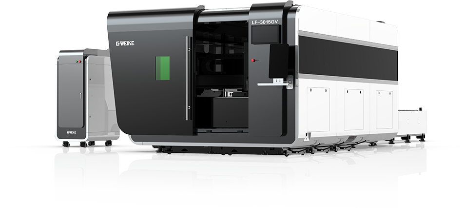
Get a timed cut on your sheet metal drawing
Send a DXF you can share, the material grade and thickness, your usual order quantity and the hole or edge requirements that decide whether the part passes. Include your preferred sheet size and assist gas if these are already fixed.
Ask for the proposed GV configuration, nest, estimated program time and a timed sample run with matching start and finish points. Review the cut quality alongside the clock before using the result in your production plan.